Demodulation of the 5G NR downlink – Daniel Estévez

On the finish of July, Benjamin Menkuec was commenting in Twitter about some points he had whereas demodulating a 5G NR downlink recording. There was a full of life dialogue during which different folks and I participated. I had by no means touched 5G, however had executed some work with LTE, so I made a decision to take the possibility to study extra in regards to the 5G bodily layer. In comparison with LTE, the adjustments are extra evolutionary than revolutionary, however understanding what has modified, and the way and why, is a part of the puzzle.
I needed to take an 11.5 hour flight in a number of days, so I thought it would be a nice challenge to offer this a shot, take with me the recordings that Benjamin was utilizing and all of the 3GPP documents, and write a demodulator in a Jupyter pocket book from scratch throughout the flight, as I had executed prior to now with my LTE recordings. This turned out to be an pleasing and attention-grabbing expertise, fairly totally different from working at dwelling in shorter intervals scattered over a number of days or even weeks, and with web entry. On the finish of the flight I had a mostly working demodulation, nevertheless it had a number of bizarre issues that turned out to be brought on by some errors and misconceptions. I labored on cleansing this up and fixing the issues over the subsequent few days, and in addition now making ready this publish.
Slightly than attempting to offer an account of all my errors and useless ends (I spoke just a little about these in Twitter), on this publish I’ll present the ultimate clear answer. There are some tough new points in 5G NR (part compensation, as we are going to see under) which may be fairly complicated, so hopefully this publish will do a superb job at explaining them in a easy approach.
The Jupyter pocket book used on this publish is here, and the recording in SigMF format may be present in this folder. Right here I’ll solely be utilizing the primary of Benjamin’s two recordings, since they’re fairly related. It was executed with an ADALM Pluto at 7.86 Msps and has a length of 143 ms. The transmitter is an srsRAN 5 MHz cell. The recording was executed off-the-air, or possibly with a cabled arrange, however there are another alerts leaking in. The SNR is excellent, so this isn’t an issue.
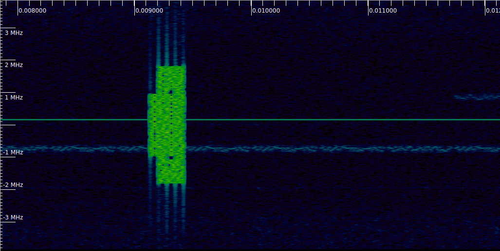
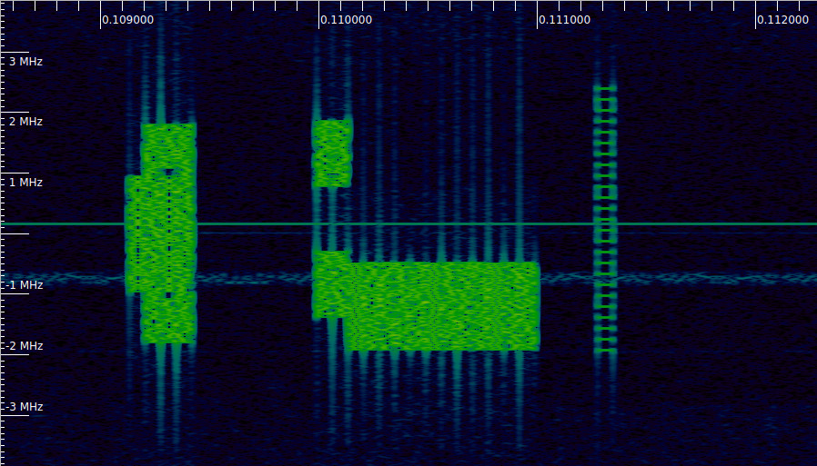
The primary sign we discover is at 9 ms. There’s a transmission like this each 10 ms. As we are going to see, that is an SS/PBCH block. One thing that stands out to these aware of the LTE downlink spectrum is that the 5G NR spectrum is nearly empty. In LTE, the cell-specific reference alerts are transmitted on a regular basis. In 5G this isn’t the case. Downlink alerts are transmitted solely when there’s visitors. There may be all the time a burst of 1 or a number of SS/PBCH blocks transmitted periodically (often each 20 ms, however on this recording each 10 ms), in addition to different alerts which can be all the time despatched periodically (such because the SIB1 within the PDSCH), however this can be all if there isn’t a visitors within the cell.
This publish assumes some familiarity with OFDM alerts and LTE. Readers unfamiliar with these may need to discuss with my LTE posts, particularly to the uplink demodulation post (not as a result of the LTE uplink has something particular to do with the 5G downlink, however relatively as a result of this was the primary publish within the collection, so it’s the place among the ideas utilized in later posts are launched).
Poor man’s Schmidl & Cox
Each time we now have an OFDM sign with a cyclic prefix and good SNR we are able to do what I name the poor man’s Schmidl & Cox. This consists in attempting to correlate the cyclic prefix in the beginning of a logo with the cyclic prefix on the finish of the identical image (they’re the identical waveform, so they need to correlate). In distinction, the true Schmidl & Cox algorithm correlates the primary half and the second half of a logo. This provides a lot better SNR as a result of longer correlation, however requires the sign to make use of solely the even subcarriers, to ensure that the 2 time area halves of the image to be equal. Some OFDM alerts which can be supposed to be synchronized with this algorithm go away odd subcarriers empty on preamble symbols, however neither LTE nor 5G do that.
The poor man’s Schmidl & Cox will give us the occasions when the symbols begin, and in addition a rough frequency estimate, computed with the part rotation over the helpful image interval. Apparently, this algorithm works inside every image, so it’s insensitive to any particular traits about how every image “connects” with the subsequent one. The traits I take into account are part rotations between every image, such because the one produced by offsetting subcarriers in frequency by half the subcarrier spacing (see the “Image inversion” part in this post), which is one thing that the LTE uplink makes use of, and in addition the brand new part compensation launched in 5G (see under). When not dealt with correctly, these options will present up as an additional, pretend, provider frequency offset when evaluating the part of the symbols as time advances. In distinction, Schmidl & Cox provides us a rough frequency estimate that ignores these errors, so it may be a superb “floor reality”.
The subsequent determine exhibits the correlation utilized to the sign proven within the Inspectrum waterfall above. The correlation peaks correspond to the places of the cyclic prefix in the beginning of every image. There are 4 symbols on this transmission, which we additionally may see by the keying clicks within the waterfall. The placement of the primary peak can be taken as the beginning of this transmission and used because the reference level for demodulation of the entire recording.

The subsequent determine exhibits the advanced values of the correlation. The frequency estimate corresponds to the angle of the correlation peaks. Right here we see that the correlations peaks are principally actual and constructive, so the frequency error is small. As in different posts, I’ve cheated, and already launched the required provider frequency offset, part offset and amplitude scale within the recording, so the estimates for these errors can be small. What I’ve executed is to use the algorithms to the recording with no corrections, compute the corrections, after which return and repeat every little thing with the corrections in place.

The provider frequency offset that I’m correcting for is eighteen.88 Hz. Apparently the Pluto was already tuned fairly precisely. After this correction, the Schmidl & Cox correlation for these 4 symbols exhibits frequency errors ranging between -6 and 42 Hz. Since that is solely a relatively coarse estimate, it’s suitable with the provider frequency error being near zero.
Part compensation
At this level we would use the image time offset obtained from the poor man’s Schmidl & Cox to carry out OFDM demodulation of the 4 symbols within the SS/PBCH block. Nonetheless, if we do that with out considering 5G’s part compensation, we are going to see bizarre frequency jumps between every image as time advances.
Part compensation is a brand new function of 5G NR in comparison with LTE, and additionally it is not utilized in different widespread OFDM waveforms. It’s a idea that may definitely be complicated. It bit me the primary time I got here throughout it, and different folks I’ve talked to additionally discover it complicated. There are possible a number of other ways to grasp part compensation, however after I attempt to consider it in ways in which must be cheap, I find yourself complicated myself. Right here I’ll attempt to clarify it in a approach that tries to encourage why it exists and tries to be the least complicated attainable. However, the part makes use of some OFDM math, so some folks may need to skip it in a primary learn.
First, let’s go to the requirements: 3GPP 38.211 defines the upconversion of a posh baseband 5G OFDM waveform (aside from the PRACH and RIM-RS), each for the downlink and uplink, as[mathrm{Re}{s_l^{(p,mu)}(t) cdot e^{2pi i f_0 (t – t^{mu}_{mathrm{start},l} – N^{mu}_{mathrm{CP},l}T_c)}}.]As standard in 3GPP’s documentation, there are a lot of technically appropriate however distracting indices and parameters. Right here (l) signifies the time area OFDM image quantity, and (p) and (mu) may be safely ignored. The provider frequency is denoted by (f_0), and (t^{mu}_{mathrm{begin},l}) signifies the beginning time of the image (l) (the beginning time of its cyclic prefix). The expression (N^{mu}_{mathrm{CP},l}T_c) provides the length of the cyclic prefix, so (t^{mu}_{mathrm{begin},l} + N^{mu}_{mathrm{CP},l}T_c) is the beginning time of the helpful image. The advanced baseband OFDM waveform (s_l^{(p,mu)}(t)) is outlined within the standard approach (once more with many unimportant variables) as[s_l^{(p,mu)}(t) = sum_{k=0}^{N_{mathrm{grid},x}^{mathrm{size},mu} N_{mathrm{sc}}^{mathrm{RB}}} a_{k,l}^{(p,mu)} e^{2pi i (k + k_0^mu – N_{mathrm{grid},x}^{mathrm{size},mu} N_{mathrm{sc}}^{mathrm{RB}}/2) Delta f (t – N^{mu}_{mathrm{CP},l}T_c – t^{mu}_{mathrm{start},l})},] for (t^{mu}_{mathrm{begin},l} leq t leq t^{mu}_{mathrm{begin},l} + T^{mu}_{mathrm{symb},l}), the place (T^{mu}_{mathrm{symb},l}) is the whole length of the image (l), together with cyclic prefix. Right here (Delta f) denotes the subcarrier spacing. That is simply your standard OFDM expression, despite the fact that it may not be instantly apparent due to the considerably complicated notation.
What’s totally different from how different OFDM waveforms work is the presence of the time period (t^{mu}_{mathrm{begin},l} + N^{mu}_{mathrm{CP},l}T_c) within the upconversion. Different OFDM waveforms together with LTE do the upconversion as[mathrm{Re}{s_l^{(p,mu)}(t) cdot e^{2pi i f_0 t}}.]This isn’t given as a formulation, however relatively as a diagram in Sections 5.8 and 6.13 in 36.211, however that is the formulation you get from the diagram.
LTE and different OFDM waveforms do the upconversion utilizing a part steady native oscillator (e^{2pi i f_0 t}). This makes good sense, as a result of in the actual world native oscillators are part steady. In distinction, 5G NR consists of the additional time period (e^{-2pi i f_0 (t^{mu}_{mathrm{begin},l} + N^{mu}_{mathrm{CP},l}T_c)}), which is totally different for every image (l) and basically causes part discontinuities within the native oscillator on the boundaries of every image, as a result of the provider frequency (f_0) multiplied by the whole image length is just not an integer (in follow transmitters don’t implement this by making use of part discontinuities to the native oscillator, however relatively by making use of the equal part rotations in advanced baseband).
Let’s again off for a second from these formulation and attempt to encourage the place the additional time period in 5G NR could come from. For this, we take into account a generic OFDM waveform with a cyclic prefix size that may fluctuate on every image. We take into account the actual case of LTE and 5G, which of their commonest configuration each have a subcarrier spacing of 15 kHz and seven symbols in every 0.5 ms interval, of which the primary one has a barely longer cyclic prefix than the remaining ones. Utilizing a notation impressed by the one in 38.211, however considerably simplified, we outline our advanced baseband OFDM image by[s_l(t) = sum_{k=-N/2}^{N/2-1} a_{k,l} e^{2pi i k Delta f (t – t_{mathrm{start},l} – T_{mathrm{CP},l})}.]Right here (N) denotes the IFFT measurement (which we assume to be even), so among the (a_{okay,l}) will usually be zero. The length of the cyclic prefix for image (l) is denoted by (T_{mathrm{CP},l}). We assume that this advanced baseband waveform is upconverted within the standard phase-continuous approach, though we are able to equivalently work in advanced baseband on a regular basis for this reasoning.
On this OFDM waveform there’s a subcarrier which is the DC subcarrier, similar to (okay = 0). Now we ask ourselves what occurs if a receiver desires to renumber the subcarriers and deal with because the DC subcarrier one other subcarrier (k_0). By this, we imply performing a frequency translation (s_l(t) e^{-2pi i k_0 t}) in order that the subcarrier (k_0) finally ends up because the DC subcarrier within the OFDM demodulation FFT. At first, this may appear only a easy renumbering of indices, and in addition considerably unjustified, however it’s neither. Allow us to first justify why a receiver could need to do that.
Suppose {that a} receiver is just on a contiguous subset of subcarriers of the complete OFDM sign, and that this subset is just not symmetric in regards to the DC subcarrier. The receiver may need to deal with as DC subcarrier the centre of this subset. There are two predominant causes for this. The primary is computational. By doing this, the receiver can compute a smaller FFT that encompasses solely the subcarriers of curiosity. Doing this requires renumbering the subcarriers, as a result of basically we are not looking for the unique DC subcarrier to be on the centre of our smaller FFT.
The second cause is extra profound. If we attempt to estimate provider part offset and image time offset in a set of subcarriers that’s skewed with respect to the DC subcarrier, we are going to discover that we are able to mistake a provider part offset for a logo time offset and vice versa. The reason being merely that the provider part offset and image time offset are given, respectively, by the impartial time period and the main time period of a level one polynomial (a straight line) that matches the part versus subcarrier measurements. If the subcarriers during which we measure are skewed with respect to zero (the DC subcarrier), then the estimates for the 2 coefficients of this polynomial are not uncorrelated. Renumbering subcarriers to deal with the centre of the set of subcarriers getting used as DC fixes this drawback.
Whereas this operation may appear as a easy renumbering of subcarriers, the next thought experiment exhibits that there’s something basic in regards to the DC subcarrier, so we can not merely deal with some other subcarrier because the DC subcarrier with out making changes. Take into account that solely the DC subcarrier is used (the remaining (a_{okay,l}) are set to zero), and that the identical image is transmitted on a regular basis (for instance, set (a_{0,l} = 1) for all (l)). Then the OFDM waveform that we get is a phase-continuous CW tone. That is true each at advanced baseband and when the waveform is upconverted to RF. If we now attempt to do the identical for a distinct subcarrier (okay neq 0), we discover that what we get has part jumps on the boundaries of every image due to the presence of the cyclic prefix (the waveform would even be a phase-continuous CW tone if there was no cyclic prefix). This exhibits that the DC subcarrier is particular. If we’re given an OFDM RF waveform, we are able to determine which subcarrier was used as DC subcarrier throughout the OFDM modulation, even when this was not in the course of the set of energetic subcarriers.
If we now work out the maths, we see that utilizing the substitutions (r = okay – k_0) and (b_{r,l} = a_{r+k_0,l}), we are able to write the frequency shifted OFDM image as[s_l(t) e^{-2pi i Delta f k_0 t} = e^{-2pi i Delta f k_0(t_{mathrm{start},l} + T_{mathrm{CP},l})} sum_{r = -N/2-k_0}^{N/2 – 1 – k_0} b_{r,l}e^{2pi i r Delta f(t – t_{mathrm{start},l} – T_{mathrm{CP},l})}.]The summation is only a common OFDM image the place the subcarriers have been renumbered in order that (k_0) is the DC subcarrier. The summation indices aren’t symmetric about (r = 0), however that is unimportant as a result of most likely we’re solely going to course of a smaller subset of subcarriers. We are able to denote this OFDM image by (widetilde{s}_l(t)). Nonetheless, along with this image, we see that we get the issue (e^{-2pi i Delta f k_0(t_{mathrm{begin},l} + T_{mathrm{CP},l})}). This depends upon the image index (l), however since we all know all of the phrases concerned, we are able to have our receiver course of the OFDM waveform as if the subcarrier (k_0) was DC, after which cancel out this further issue by making use of a part correction that depends upon (l).
In sensible conditions the part correction is kind of manageable. If there’s an integer (L) such that the length of (L) consecutive symbols multiplied by (Delta f k_0) is an integer, then we see that the part correction relies upon solely on (l) modulo (L). For the standard 15 kHz subcarrier spacing of LTE and 5G, we are able to all the time take (L = 14), and in addition (L = 7) if (k_0) is even. The part corrections may even be precomputed as a desk of size (L), and the right time period may be utilized by realizing the image index throughout the group of (L) consecutive symbols.
Nonetheless, one thing essential in all of that is that thus far we now have assumed that the receiver is aware of the index (k_0), or equivalently, that it is aware of what’s the subcarrier that the transmitter used as DC. Think about an OFDM waveform that doubtlessly has numerous subcarriers, however often solely a small portion of them (not centred in regards to the DC subcarrier) are in use. A receiver may detect the presence of the waveform due to the subcarriers which can be energetic. Nonetheless, it may not know the relative place that these subcarriers occupy within the frequency grid of the complete OFDM waveform. In different phrases, it may not know the indices (okay) of the subcarriers that it has detected. On this case, it can not apply the part correction and function with the set of energetic subcarriers by treating certainly one of them as DC. I don’t know a lot in regards to the system ranges necessities of 5G, however I believe that this example is taken into account as a use case.
The part compensation of 5G solves this drawback. If as an alternative of upconverting our advanced baseband OFDM waveform as (mathrm{Re}{s_n(t) e^{2pi f_0 t}}) we upconvert it as (mathrm{Re}{s_n(t) e^{2pi f_0 (t – t_{mathrm{begin},l} – T_{mathrm{CP},l})}}), we are able to repeat the identical sort of calculation and see that when the receiver downconverts this RF waveform by multiplying by (e^{-2pi i (f_0 + Delta f k_0) t}), the advanced baseband waveform that it’ll receive is[e^{-2pi (f_0 + Delta f k_0) ( t_{mathrm{start},l} + T_{mathrm{CP},l})} widetilde{s}_l(t).]Now the part correction time period that it wants to use depends upon (f_0 + Delta f k_0), and that is an absolute RF frequency. It’s not relative to the subcarrier that was used as DC within the transmitter. It’s the nominal RF frequency of the subcarrier that the receiver desires to make use of as DC. So long as the receiver provider frequency offset is just not too massive, it could determine the nominal provider frequencies of the energetic subcarriers that it has detected.
There are a few extra remarks that assist encourage precisely why these specific part jumps are used within the 5G part compensation, apart from the rationale “in order that the maths works out within the receiver”. The primary is that each one the subcarriers of a posh baseband OFDM waveform have their part aligned at zero in the beginning of the helpful image (simply consider the definition). The 5G part compensation time period is the required expression in order that this property can also be true for the subcarriers within the upconverted waveform. The second comment is that the 5G OFDM waveform can truly be seen (a minimum of within the case during which (f_0) is an integer a number of of (Delta f)) as an OFDM waveform whose DC subcarrier is definitely at RF DC, and the set of used subcarriers is approach up within the RF vary across the supposed provider frequency. On this sense, not one of the energetic subcarriers is particular (none are the DC subcarrier), and a receiver can determine the subcarrier index (okay) of every of them by measuring their RF frequency.
In follow, to deal with the part compensation for the recording used on this publish, we have to know that the subcarrier that’s near 0Hz within the recording (which we are going to use as DC) has a nominal frequency (f_{mathrm{DC}}) of 1876.95 MHz. As soon as we all know this, and taking benefit that this provider frequency is a a number of of two kHz, we are able to construct a desk of (L = 7) part corrections, and apply them relying on the image index modulo 7. Our desk of part corrections can have a continuing part error, since this can be absorbed by the receiver part error. Due to this fact, we merely construct the desk as (e^{2pi i f_{mathrm{DC}} T_{mathrm{CP},1} l}), for (l = 0, 1, ldots, 6). Right here (T_{mathrm{CP},1}) denotes the length of the cyclic prefix of all symbols besides the primary in every group of seven (which has a slighly longer cyclic prefix).
The SS/PBCH block
Now that we all know in regards to the 5G NR part compensation, we are able to demodulate the 4 symbols within the transmission that we’re analysing, which is an SS/PBCH block. The SS/PBCH block is the substitute in 5G for the LTE PSS (major synchronization sign), SSS (secondary synchronization sign) and PBCH (bodily broadcast channel). The SS/PBCH block additionally accommodates the PSS, SSS, and PBCH, however every of those is considerably totally different from their LTE counterparts.
The next diagram exhibits the time-frequency construction of the SS/PBCH block. Observe that this seems identical to what we noticed in Inspectrum. The block consists by 4 consecutive OFDM symbols. The beginning image of the block is both image 2 or image 8 (utilizing zero-based numbering) in a 1 ms subframe, so not one of the symbols have the marginally longer cyclic prefix of symbols 0 and seven. In distinction with LTE, the SS/PBCH block may be transmitted wherever within the cell frequency grid. It doesn’t have to be centered in regards to the DC subcarrier.
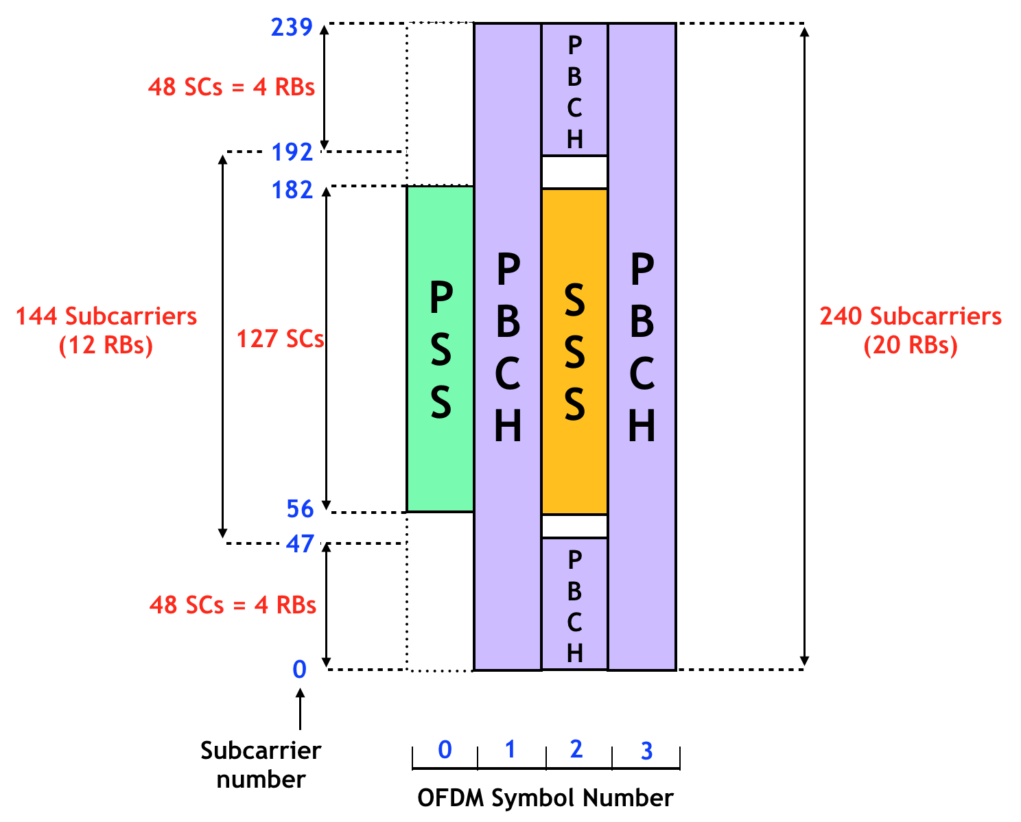
The PSS and SSS are BPSK modulated utilizing pseudorandom sequences that depend upon the cell ID. This contrasts with LTE, the place the PSS is a Zadoff-Chu sequence. The 5G cell ID is outlined as in LTE, as (N_{mathrm{ID}}^{mathrm{cell}} = 3 N_{mathrm{ID}}^{(1)} + N_{mathrm{ID}}^{(2)}), though the vary of attainable values for (N_{mathrm{ID}}^{(1)}) is from 0 to 335 (in LTE it was from 0 to 167). The attainable values of (N_{mathrm{ID}}^{(2)}) are nonetheless 0, 1, and a pair of. As in LTE, the PSS solely depends upon (N_{mathrm{ID}}^{(2)}), so there are solely 3 attainable waveforms to seek for cell discovery, after which as soon as (N_{mathrm{ID}}^{(2)}) is know, we are able to discover (N_{mathrm{ID}}^{(1)}) from the SSS. The pseudorandom sequences used for the development of the PSS and SSS are primarily based on m-sequences of size 127, so this explains why they use 127 subcarriers.
As proven within the determine above, the PBCH is transmitted across the SSS. That is totally different from LTE, the place the alerts have been transmitted sequentially in time (first SSS, then PSS, then 4 PBCH symbols). The PBCH has its personal DM-RS (demodulation reference sign), as a result of there are not any cell-specific reference alerts energetic on a regular basis as in LTE. The PBCH DM-RS occupies the subcarriers whose index is congruent with the cell ID modulo 4.
PSS
To demodulate the PSS, and the opposite alerts within the SS/PBCH block, we have to know the subcarrier index at which the SS/PBCH block begins. In our case we are able to do that simply by which subcarriers are energetic. The next determine exhibits the facility of all of the subcarriers after OFDM demodulation of the PSS. Utilizing this we discover that the SS/PBCH block begins at subcarrier -120 with respect to the subcarrier that we now have chosen to make use of a DC subcarrier.

Right here is the constellation of the PSS. All the pieces seems good, as a result of as I’ve talked about, I’m dishonest and have already utilized the provider frequency, part and amplitude corrections required.

The three attainable PSS sequences (relying on (N_{mathrm{ID}}^{(2)})) are round shifts of a 127-bit m-sequence. In our case we are able to merely discover that (N_{mathrm{ID}}^{(2)} = 1) by trial and error. After wiping off the sequence, we receive the next constellation. Right here the image time offset comes from the poor man’s Schmidl & Cox, and it has a decision of 1 pattern, so there’s a little of sub-sample image time offset. This can be corrected later. Additionally, we see that one of many subcarriers is considerably off. That is brought on by a CW interference, which may be seen within the waterfall or within the spectrum above.

That is often not how a receiver makes use of the PSS, as a result of right here we now have began with a relatively good image time offset by utilizing the poor man’s Schmidl & Cox. Normally, a time area correlation is finished with the three attainable PSS symbols to search out the placement of the beginning of the PSS (which supplies us the image time alignment) and the (N_{mathrm{ID}}^{(2)} = 1). In doing this, the right frequency offset must be used when producing the time-domain PSS waveform. The outcomes of doing this are proven within the subsequent plot.

SSS
We are able to receive the SSS by demodulating two symbols after the PSS. Right here you will need to use the 5G part compensation correction accurately, or we might get a bizarre part bounce between the PSS and SSS that may lead us to assume that there’s a provider frequency offset. The constellation is proven right here.

The SSS sequence relies upon each on (N_{mathrm{ID}}^{(2)}), which we already know, and on (N_{mathrm{ID}}^{(1)}), which we don’t. There are two attainable methods to search out the right SSS sequence, and with it, the worth of (N_{mathrm{ID}}^{(1)}). The primary is brute power correlation in opposition to the sequences for all of the attainable values of (N_{mathrm{ID}}^{(1)}). The result’s proven right here. We see that (N_{mathrm{ID}}^{(1)} = 0), so the cell ID is 1.

As within the case of LTE, there’s a cleverer extra environment friendly approach that exploits the development of the SSS sequence. The SSS sequence is a Gold-code-like sign that’s constructed from two 127-bit m-sequences (x_0) and (x_1). The SSS sequence is the XOR of (x_0) circularly shifted by (m_0) positions and (x_1) circularly shifted by (m_1) positions. Whereas (m_1 = N_{mathrm{ID}}^{(1)} mod 112), the nice factor is that[m_0 = 15 leftlfloorfrac{N_{mathrm{ID}}^{(1)}}{112} rightrfloor + 5N_{mathrm{ID}}^{(2)}.]Since we all know (N_{mathrm{ID}}^{(2)}), there are solely 3 potentialities for (m_0).
What we are able to do is, for every risk of (m_0), XOR the obtained SSS with (x_0) shifted by (m_0), in order that solely the contribution of (x_1) stays, after which carry out a round correlation between this and (x_1) to acquire (m_1). The round correlation may be executed effectively with FFTs (although such an FFT is difficult to implement, as a result of 127 is prime). From the values of (m_0) and (m_1) we are able to get well (N_{mathrm{ID}}^{(1)}). The results of this method is proven right here.

After wiping off the SSS sequence, we receive the next constellation.

OFDM demodulation
At this level I’ve carried out the OFDM demodulation of all of the symbols within the recording. On this demodulation I’m additionally considering a sampling frequency offset and effective image time offset (which can be estimated under). The time offset for every image is decomposed as an integer variety of samples, which may be utilized by selecting the beginning pattern for OFDM demodulation, and a sub-sample delay, which is utilized as a part slope within the frequency area after OFDM demodulation.

Moreover, right here and within the earlier OFDM demodulations I’m beginning the demodulation on the center of the cyclic prefix relatively than in the beginning of the helpful image for max robustness in opposition to image time offset errors. This additionally must be compensated as a part versus frequency slope after demodulation.
To demodulate all of the OFDM symbols correctly, you will need to know which is the primary image in every 0.5 ms half-subframe, as a result of it has a barely longer cyclic prefix, and since the part compensation correction resets at these symbols. Since within the recording we’re utilizing there’s a single SS/PBCH block per 10 ms radio body, we all know that this block begins at image 2 of the primary subframe of every radio body.
PBCH
As talked about above, the PBCH occupies three symbols within the SS/PBCH block (certainly one of these symbols is shared with the SSS), and one out of each 4 subcarriers is used as DM-RS. Each the PBCH knowledge and its DM-RS are QPSK modulated. The DM-RS sequence is generated with the generic pseudorandom sequence algorithm, which is similar as in LTE, a (2^{31}-1) bit Gold code (utilizing a 31-bit register). The preliminary worth for the Gold code is[c_{mathrm{init}} = 2^{11}(overline{i}_{mathrm{SSB}}+1)(lfloor N_{mathrm{ID}}^{mathrm{cell}} / 4 rfloor + 1) + 2^6 (overline{i}_{mathrm{SSB}}+1)(N_{mathrm{ID}}^{mathrm{cell}} mod 4).]Right here (overline{i}_{mathrm{SSB}}) basically is the index of the SS/PBCH block in a ten ms radio body (it counts repetitions of the SS/PBCH block in the identical radio body). Utilizing a distinct DM-RS for every repetition of the SS/PBCH block permits the receiver to determine which repetition it’s processing, by blind looking out the DM-RS, and so to acquire time synchronization to the radio body. On this recording there is just one SS/PBCH block per radio body, so (overline{i}_{mathrm{SSB}}) is all the time zero.
With this information we are able to demodulate the PBCH and wipe-off the sequence for the DM-RS. The next determine exhibits the constellations of the three alerts in every SS/PBCH block within the recording (there are 13 of them, the primary one showing at ~9 ms, and the final one at ~139 ms). Every SS/PBCH block corresponds to a row within the determine. The PSS and SSS are proven with the sequences wiped off within the first and second columns respectively. The PBCH and its DM-RS are proven within the third column. The info symbols are plotted in blue, and the wiped-off DM-RS symbols are plotted in inexperienced.

Since I’ve adjusted the provider frequency offset, part offset, amplitude, sampling frequency offset and image time offset, the OFDM demodulation stays properly synchronized all through all of the recording.
Image time offset
To regulate the preliminary image time offset extra finely than what obtained with the poor man’s Schmidl & Cox, and to find out the sampling frequency offset, I’ve used the demodulated PSS to measure the part versus frequency slope by becoming a polynomial of diploma one to the part of the wiped-off PSS subcarriers. The ensuing image time offset is proven right here.

This plot has been obtained already correcting for preliminary image time offset and sampling frequency offset, so the ensuing time offset is near zero. To acquire these parameters, a polynomial of diploma one is fitted to this plot. The impartial time period provides the preliminary image time offset, and the main coefficient provides the sampling frequency offset, which is -3.2 ppm for this recording.
Moreover, to examine the channel response, I’ve plotted the part of the subcarriers of the primary 4 PSS symbols. The part is kind of flat, as must be the case with a channel with out multipath or dispersive results (the spike is brought on by the CW interference).

Different alerts within the recording
Lastly, I’ve turned my consideration to the remainder of the alerts within the recording. Since there aren’t many, I can go manually over every of them. To find the alerts shortly, I’ve plotted the whole sign energy in every image, categorized by radio body. Every row of the plot corresponds to a radio body. Symbols within the radio body observe the unconventional method of beginning on the PSS, since that is the primary image I’ve demodulated. The PSS must be image quantity 2 (with zero-based indexing) within the body. This distinction is just not essential, specifically as a result of there are by no means any alerts in symbols 0 and 1 on this recording.

We see that the SS/PBCH block seems in the identical place in every radio body. It is usually attention-grabbing to see the variations in sign energy of the 4 symbols within the SS/PBCH block. These are precipitated as a result of a distinct variety of subcarriers are in use in every image (since every subcarrier has all the time the identical energy, the whole energy we see is proportional to the variety of energetic subcarriers).
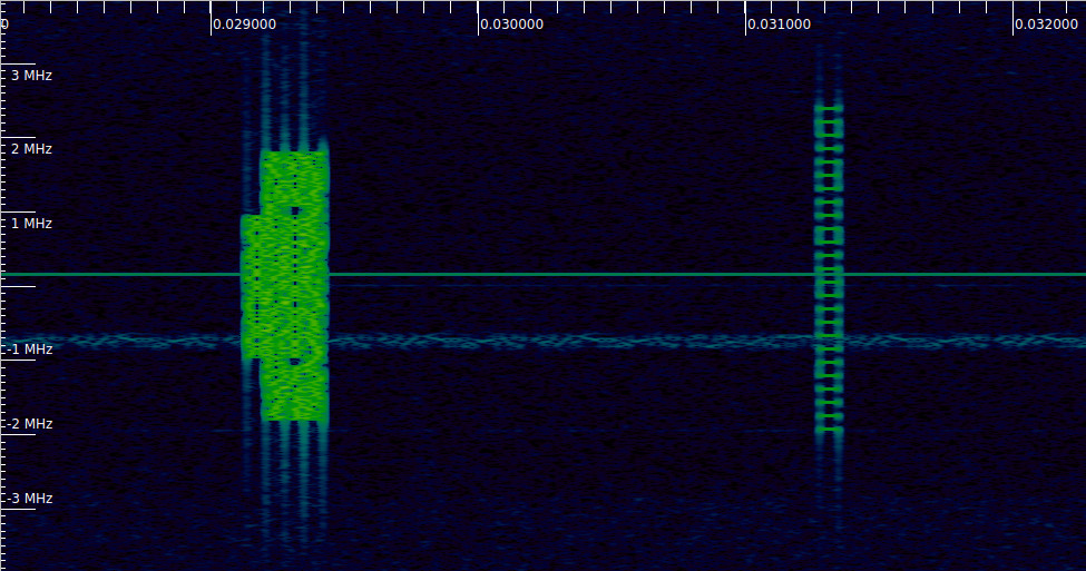
Most radio frames solely comprise the SS/PBCH block, however a number of frames comprise different alerts. Body quantity 2 accommodates a sign that occupies a single image. It seems in image 32 within the radio body (correctly counting the PSS as image 2), which is image 4 in subframe 2. Wanting on the waterfall, we see that the subcarriers are sparsely used. The truth is, just one in each 12 subcarriers is energetic. The identical sort of sign seems in the identical place in body quantity 10.
I haven’t tried too exhausting to determine every of the alerts on this part, since I’m not but too aware of the entire zoo of 5G NR alerts. The 3GPP paperwork aren’t the most effective to determine them, because it’s simple to get misplaced within the notation. A ebook or webpage with some diagrams and examples is a a lot better useful resource.
On this case, whereas analysing the recording throughout my flight, I famous down that these are possibly the PDCCH DM-RS alerts, since 38.211 Part 7.4.1.3.2 says that they use one subcarrier in every useful resource block (i.e., each 12 subcarriers). Nonetheless, in hindsight that is considerably unusual, as a result of there are not any accompanying PDCCH knowledge symbols. Possibly the PDCCH can simply be empty, however its DM-RS must be current. Or maybe that is some sort of “channel sounding” reference sign (such because the CSI RS). It is going to be good to come back again to those alerts in a future publish and determine them correctly. The constellation plots of those two alerts are proven right here. They’re QPSK modulated.


In body 3 there are alerts that use 4 OFDM symbols. They seem in symbols 32, 36, 46, and 50 within the radio body, that are symbols 4 and eight in subframes 2 and three. They use one out of each 4 subcarriers.
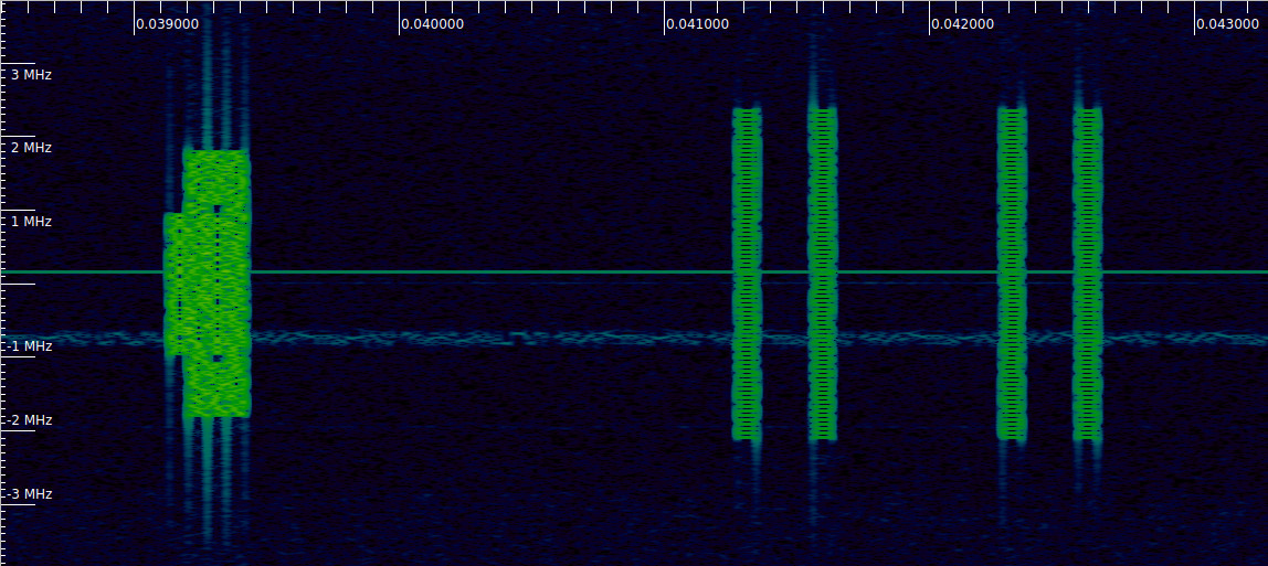
The constellation plots for these alerts are proven right here. Every OFDM image is proven in a distinct sq. within the 2×2 grid. In my flight I took word that possibly these are some sort of reference sign, since they use the subcarriers sparsely.


Radio body 10 is the busiest. Moreover the identical sign as in body 2, we see a number of different alerts.
The primary of those alerts occupies two symbols within the time area, and two segments of 6 useful resource blocks with a niche of 6 useful resource blocks within the frequency area. The symbols utilized by these sign are 14 and 15, that are the primary and second image in subframe 2. Throughout my flight I took word that possibly that is the PDCCH, although I’m undecided about this. Observe that if that is the truth is the PDCCH, then it doesn’t make a lot sense for the sparse refrence sign to be the PDCCH DM-RS, as a result of it’s fairly far aside in time.

The subsequent sign occupies 8 useful resource blocks within the frequency area, and 12 symbols within the time area (symbols 2 to 13 in subframe 2). The sign in symbols 2, 7, and 11 is totally different. It solely makes use of each different subcarrier and its amplitude is (sqrt{2}) as an alternative of 1. I believe that is the PDSCH, and the particular symbols are its DM-RS. I’ve marked them as such within the determine under. All of the symbols are QPSK modulated.

There are not any extra alerts within the recording. Most likely at this level I’ve some folks yelling at me that I’ve misidentified a few of these alerts, however this appears a great way of discovering out what they really are. In any case, finally I’ll learn extra about 5G and are available again and do a correct classification.